During my master’s I started collecting a list of quantum information problems that can be either solved or approximated with convex optimization. For obvious reasons (e.g., because quantum states and measurement effects are semidefinite operators satisfying linear constraints), semidefinite programming often pops up. Frequently, though, it is more difficult (and takes much more time) to actually solve those problems in practice than to understand them. Some of the many reasons are that (i) there is no one-size-fits-all set of tools and that (ii) you need to know at least the very basics of programming to be able to (iii) figure our the programming patterns that often appear in quantum information problems and to (iv) make sense of all the tools available and decide which to use.
It would have saved me a lot of time to have more code examples when I started, and that is one of the reasons why I collected these simple applications of semidefinite programming to quantum information problems.
(Note: I’m assuming you know what a semidefinite program is. If you don’t, take a look at this paper or, for a more quantum informational perspective, this chapter in Watrous lecture notes.)
For a start, I will talk about some of the terminology and tools availables, with some tips of what you should look for when choosing a programming language, a solver and a modelling system. Then I will show some very simple examples implemented in several languages: PPT criterion for entanglement (Mathematica), joint measurability (Julia) and using a see-saw to maximize the violation of Bell inequalities (Python). If you already know all about that, in the end I discuss a more interesting example: how to implement a symmetric extensions hierarchy (with bosonic symmetry) that can certify the Schmidt number of a density operator.
Time allowing, I will update this with my collection of SDPs in QI when I get to tidy up the codes or implement new ones…
Tools
Many tools, free and paid, can help in solving optimization problems. It is important to have an overview of them because, as always, there are trade-offs in each choice: a more expressive programming language requires less coding and is easier to understand, but generally slower; the most natural mathematical expression of a program is not always the best way to code it etc. Knowing what you need to implement will often trim down your choice to one of a few sets of tools.
Programming languages
Many programming languages are commonly used to solve optimisation problems. Roughly in increasing order of “difficulty” to use are MATLAB, Python, Julia, Fortran and C. Mathematica is seldom used (mainly because it is slow, black-boxed and has few good packages for dealing with common patterns in optimisation), but it has it’s usefulness for simple prototyping.
(Note: The ones listed above are general-purpose programming languages that you can use for optimisation, but many other things. Apart from them, there are also the so-called “modelling languages”, which are tuned specifically for mathematical optimisation. Famous ones are AMPL and GAMS. As I understand, they are routinely used in the industry, but I have no experience with them and haven’t heard of anyone using it in quantum information.)
Solvers
These are the softwares that implement the algorithms to solve optimization problems. They are usually implemented in low-level languages and many different options (both open-source and commercial) exist for each types of optimization programs (linear programming, cone programming, nonlinear programming etc.) If all you care about is solving some small to medium-sized instances of optimization problems, you don’t have to care much about learning how the algorithms work, much less about doing your own implementations. These are very complicated programs, and highly optimized for speed, so the chances you’d come up with a better implementation are very slim anyway.
Linear programming
- Gurobi is frequently used for linear programming (although it can deal with other types of programs, such as quadratic programming and mixed-integer programming). It is proprietary but has free academic licenses (even if you want to set-up a license server in a cluster). It is very fast and a generally good choice for large programs.
- HiGHS is open source and and has comparable performance.
- Other options include GLPK and many of the SDP solvers, such as ECOS.
Semidefinite programming
- MOSEK is frequently used for SDPs (and one of the fastest and most robust options), but it can also solve quadratic programs, second-order cones and mixed-integer programs. Similarly to Gurobi, it is proprietary but provides academic licenses for single and cluster users. Although it is a remarkably fast solver (w.r.t. its precision), very large problems will require a lot of memory. In that case, you may try…
- SCS, which is open-source and implements a different method than MOSEK, one that requires less memory but perhaps running time (if you crank the precision to match those of MOSEK). With the default parameters, though, it performs comparably well, and the results are more than good enough for our use cases. For too large problems, this may currently be the only viable option.
- SDPA, SDPT3 and SeDuMi are also common choices with comparable performance.
Performance comparison
Here are some performance comparisons of popular solvers:
- Sparse SDPs comparing MOSEK, SDPA, SeDuMi, SDPT3 and others.
- Linear programming via simplex method comparing Gurobi, MOSEK, GLPK etc.
- Linear programming via barrier methods comparing Gurobi, MOSEK, HiGHS etc.
Modelling systems
When you write an optimisation program on paper, it usually looks quite different from the “standard form” that a solver expects to be handed. This means that dealing directly with your solver is quite cumbersome and involves a lot of reformulations. For instance, you would have to put your complex variables into polar form to convert it to a real formulation, you would have to write your own routines to represent Kronecker products, traces and other common operations etc. Even worse, it is common to try out different solvers for a same problem, and since each of them works differently, you would have to rewrite everything in case you wanted to change solver midway through an implementation.
That is one of the reasons why people created many packages to do this conversion automatically. Some of them, for the programming languages above, are:
- MATLAB: YALMIP, CVX
- Python: CVXPY, PICOS, Pyomo
- Julia: JuMP.jl, Convex.jl
- C and Fortran: In this case I think you’d be fine finding your own libraries 🙃.
Because in quantum information we commonly use uncommon linear operations, you better do some planning on which packages to choose before you start writing your program, or you’ll end up having to manually code all of them. Basically, you should look for (at least) support for complex numbers, partial trace, partial transpose and kronecker product.
CVX, together with QETLAB, is the way to go if you’re into MATLAB. In Python, there are more options: At least PICOS and CVXPY have kronecker product, partial trace and transpose implemented (PICOS was a first on this). In Julia, Convex.jl has them, and it is in many ways similar to the Python options.
Another thing to keep an eye on is that some of these modelling systems are specialised for some types of optimisation problems (e.g. cone programming), while others are more general (JuMP.jl). On the bright side, specialised systems will do some checking on your formulation, raise warnings if you mess something up, and are usually a bit higher-level. On the other hand, all these features induce some overhead, so for enormous programs you might want to go a bit lower-level.
(Note: If you have some sizeable programs to solve and neither of the options above can deal with it, you might go for Julia with JuMP.jl (it’s memory footprint is way smaller than Convex.jl, for instance). Even though it doesn’t have complex number support yet, you can do some patchworking with ComplexOptInterface.jl, and then reuse Convex.jl implementation of partial trace and partial transpose. Take a look at the Schmidt number computation later on to see an example.)
Entanglement via PPT criterion (Mathematica)
Any bipartite separable state $\rho$ can be written as
$$ \rho = \sum_i p_i \rho_A^i \otimes \rho_B^i . $$
Taking the partial transpose in any of the subsystems (e.g. in the second), we get
$$ (I \otimes T)\rho = \sum_i p_i \rho_A^i \otimes (\rho_B^i)^\intercal $$
Because the eigenvalues of the tensor product is the product of eigenvalues, and because transposition leaves $\sigma(\rho_B^i)$ unchanged, then the spectrum of $\rho$ and $(I \otimes T)\rho$ are the same. Moreover, we know that all eigenvalues of $\rho$ are nonnegative. This implies that if $\rho^{\intercal_B}$ has a negative eigenvalue, then $\rho$ is entangled. (The same is valid for $\rho^{\intercal_A}$, since it is equal to $(\rho^{\intercal_B})^\intercal$.
This was first observed in this paper Peres’ “Separability criterion for density matrices” and soon thereafter shown to be a sufficient criterion for $2 \times 2$ and $2 \times 3$ systems in the Horodeckis’ “Separability of mixed states: necessary and sufficient conditions”.
Naturally, the PPT criterion can be tested in a very simple manner, without the need for any optimization. However, it is still useful to notice that enforcing $\rho \geq 0$ is a constraint compatible with SDPs, thus we can optimize all sorts of functions over the set of PPT entangled (or separable/bound entangled) states.
One simple application of SDPs is to take a parametrized state, such as the $2$-qubits isotropic state
$$ \rho = \alpha \ket{\Psi^+}\bra{\Psi^+} + (1 - \alpha) \frac{I_4}{4} $$
and search for the highest visibility $\alpha$ such that is it still separable. Because the PPT criterion is necessary and sufficient for $2 \times 2$ states, the solution will give us exactly the separable/entangled transition.
I wrote a solution to this in Mathematica, together with a slightly more interesting problem, in this .nb.
Joint measurability robustness (Julia + Convex.jl)
Quantum measurements can be incompatible. Among several definitions, one of clear operation meaning is the one of joint measurability: Two measurements $A$ and $B$ are jointly measurable if there exists a parent measurement $G$ such that, through classical pre- and post-processing, the statistics of $A$ and $B$ can be reproduced. Equation-wise, we want to find a set of operators
$$ G = { G_{ab} }_{a=1,b=1}^{n_A,n_B} $$
such that $\sum_{ab} G_{ab} = I$ and $G_{ab} \geq 0, ,\forall a, b$ (i.e., $G$ is a well-defined quantum measurement) and
$$ \sum_b G_{ab} = A_a ;;\text{ and };; \sum_a G_{ab} = B_b . $$
Going one step further, we can also try to quantify how incompatible $A$ and $B$ are. This can be done via the incompatibility robustness (which is nicely discussed in Designolle et al.’s “Incompatibility robustness of quantum measurements: a unified framework”.
Simplifying it a bit, what we want is to mix $A$ and $B$ with some sort of noise until they become jointly measurable. A simplest choice of noise is the random noise. So we want to maximize $\alpha$ such that
$$ \sum_b G_{ab} = \alpha A_a + (1 - \alpha) \frac{I}{n_A} ;\text{ and } \sum_a G_{ab} = \alpha B_b + (1 - \alpha) \frac{I}{n_B} $$
Together with the PSD conditions on $G$, this is a semidefinite program. Here’s a solution (for two measurements) using Julia + Convex.jl:
| |
The curve below is what you get. Notice that I’ve chosen a set of measurements for which an analytical solution is known, so that you can see it exactly matched the SDP solution (as it should). For more general measurements (we can also generalize the definition to dealing with more than two measurements, as in Appendix E of the paper), optimization is the only way.
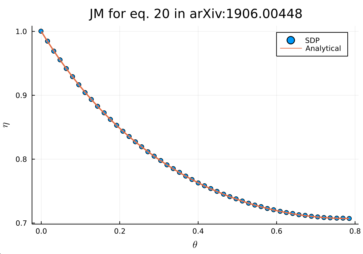
Joint measurability via SDP.
Violation of tilted CHSH inequality (Python + PICOS)
In a nonlocality scenarios, we frequently want to find the maximum quantum violation of some Bell inequality. As we will see, this is not an SDP (our objective function will turn out to be nonlinear), but we can approximate the solution using a procedure called see-saw (or alternated optimization), which is very useful to know.
Let us start from the tilted CHSH inequality, analysed in Acín et al.’s “Randomness versus nonlocality and entanglement”,
$$ \alpha \langle A_0 \rangle + \langle A_0 B_0 \rangle + \langle A_0 B_1 \rangle + \langle A_1 B_0 \rangle - \langle A_1 B_1 \rangle \overset{C}\leq 2+\alpha \overset{Q}\leq \sqrt{8+2\alpha^2} $$
In this expression, the $C$ bound is the local bound (i.e., achievable with classical systems), and the $Q$ bound is the analytical solution for the maximum violation using quantum systems. (Of course, in general we don’t know the quantum bound for all inequalities, I just picked this example so we can compare the curve we will obtain via optimization.)
Applied to quantum systems, what we want is to find the best measurements $A_0$ and $A_1$ on Alice’s side and $B_0$, $B_1$ on Bob’s side, together with the best shared quantum state $\rho_{AB}$, such that we maximize the l.h.s. of the inequality. In quantum theory, the expectation values can be written as
$$ \langle A_i B_j \rangle = \text{tr}(\rho_{AB} \cdot A_i \otimes B_j). $$
We can define
$$ G \equiv \alpha A_0 \otimes I_B + A_0 \otimes B_0 + A_0 \otimes B_1 + A_1 \otimes B_0 - A_1 \otimes B_1 $$
as, from linearity, write that we want to find $\max \text{tr}(G \rho_{AB})$ such that
$$ \text{tr} \rho_{AB} = 1 ;\text{ and } \rho_{AB} \geq 0 $$
and $A_i$, $B_i$ are well-defined measurements (PSD operators and sum to identity). This feasible set is totally fine for an SDP, but our objective function is not, for both the measurements and the state are variables, making the whole thing nonlinear. We can simplify it a bit by noticing that, for fixed measurements, the optimal state is the maximal eigenvector of $G$, but we are still left with $A_i \otimes B_j$ being nonlinear when both are variables. What we can do, then, is a see-saw procedure:
- Randomly sample initial measurements and take the optimal $\rho$.
- Optimize over Alice’s measurements while keeping Bob’s constant.
- Optimize over Bob’s measurements while keeping Alice’s constant.
- Update the optimal $\rho$
- Repeat from $2$ until convergence.
On the bright side, we can get nice lower bounds for quantum violations in such way. However, because we are not just solving a single SDP anymore, we lose our global optimality guarantees. Even worse, the final result is highly dependent on how well you made your initial guess of measurements. What people usually do, then, is to run this algorithm for many different initial conditions, and take the best shot as the solution. Thus, if all you want to do if to prove some Bell inequality can be violated with quantum systems, this is a way to go, but you will in general not find the optimal violation.
Remark: There is a way to also approximate the quantum behaviors from the outside of the set through a hierarchy of SDPs (the NPA hierarchy). That gives upper bounds on the maximal quantum violation. If you apply a see-saw and an NPA to the same inequality and find the same number, then you can guarantee that’s the actual quantum bound.
Here is an implementation of this algorithm in Python + PICOS, and the result you get for a modest number of initial settings.
| |
To highlight the fact that global optimality is lost, I ran this for a small number of settings, so you can see we only get lower bounds (for this particular case, it is easy to get closer to the actual curve):
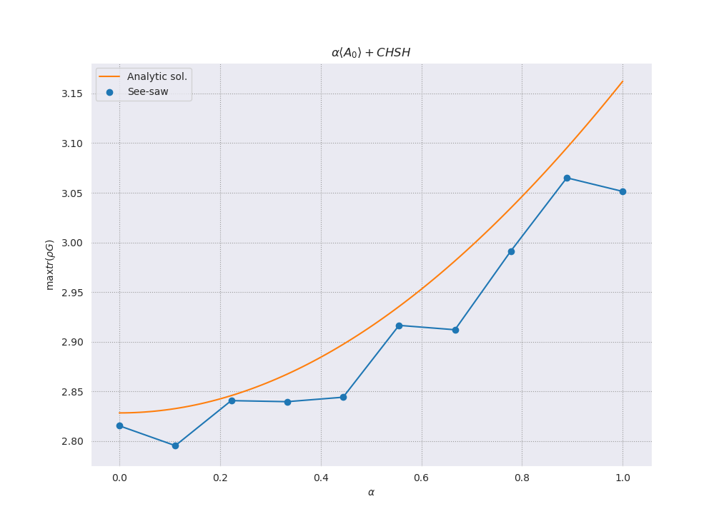
Tilted CHSH violation with a see-saw procedure.
Schmidt number certification (Julia + JuMP.jl + ComplexOptInterface.jl)
At least in principle, the DPS hierarchy (if you’re into that, you might also be interested in reading about the quantum inflation technique and entanglement between cones) can completely solve the separability problem (of course, as the experimentalists say, “in practice the theory is different”).
In a nutshell, the arguments goes as this: If $\rho_{AB} \in \mathcal{L}(H_A \otimes H_B)$ is separable, then we can take $N$ copies of the $B$ subsystem and write $$ \Xi = \sum_i p_i \rho_A^i \otimes (\rho_B^i)^{\otimes N} . $$
So, if we pick some $N$ and find out it is impossible to write a $Q$ such that $$ \rho_{AB} = \text{tr}_{(B)_i : i \in [N] \setminus m}\left( \Xi \right) , \forall m $$
this means $\rho_{AB}$ is entangled.
In the paper, they also prove this hierarchy is also complete, in the sense that a symmetric extension to any order $N$ exists if and only if $\rho_{AB}$ is separable. Of course, in practice, we can only go so high on $N$, and not very: Take a look at the dimension of the resulting operator… To mitigate that, in the paper they also argue that symmetric extensions live in $\text{Sym}_N(\mathcal{L}(H))$, which is actually only of dimension
$$ d_{\text{Sym}_N} = \text{binomial}(d_B + N - 1, N) . $$
This means we can actually go reasonably far in the hierarchy, which is quite cool. What is even cooler is that we can use an extra piece of information to transform this into not only an entanglement certificate, but also a Schmidt number lower-bound certificate.
The key fact comes (to the best of my knowledge) from this paper about optimizing Schimdt number witnesses (more recently, the same observation was made in this other paper about faithful entanglement): Any pure state $\ket{\psi} = \sum_{i=1}^k \eta_i \ket{\alpha_A, \beta_B}$ can be expressed as
$$\ket{\psi} = \Pi^\dag_k \left( \ket{\alpha^\prime_{AA^\prime}} \otimes \ket{\beta^\prime_{B^\prime B}} \right),$$
i.e., as a separable (unnormalised) operator w.r.t. the $AA^\prime / B^\prime B$ partition in a “lifted” space. Here, $\Pi_k = \eye_A \otimes \sum_{i=0}^k \ket{ii}_{A^\prime B^\prime} \otimes \eye_B$ is something like an “entangling projection” between the primed subsystems.
In practical terms, this means that any $\rho_{AB}$ with Schmidt number $k$ (or less) can be mapped to a trace-$k$ separable operator. So, we might as well check if the $B^\prime B$ can be symmetrically extended to some order $N$. If it cannot, this means $\rho_{AB}$ has Schmidt number larger than the $k$ we tried.
If we want to precisely determine $k$, we end up with a double hierarchy (on both the Schmidt number and the extension order). On top of that, we also significantly increase the Hilbert space dimension, since we have to add two $k$-dimensional subsystems (the primed ones). Obviously, then, we cannot go very far with this, but it works OK for some cases (up to local dimension $5$ I can test $k > 2$ of a GHZ state on a decent computer.)
The full implementation of this one requires some utility functions (e.g., to project onto the symmetric subspace etc.), but the main routine goes as follows:
| |
You can find the full thing here.